R Deep Dive Series - R2jags
Kelsey Martinez, PhD, Researcher
August 19, 2020

Photo by Safar Safarov
Bayesian analytical approaches are becoming more and more common in the data science world. Why is that? Aren’t Frequentist approaches confusing enough to interpret? Bayesian approaches are particularly useful in some applications because they allow the analyst to inform the modeling process more than some frequentist approaches. For example, using hierarchical Bayesian approaches, we can model much more complex processes as compared to many Frequentist approaches. More on hierarchical models can be found here.
Bayesian models also produce posterior distributions with 95% credible intervals to determine relationships between variables, while the Frequentist approach uses the all-too-familiar p-value & alpha cut-off levels for determining statistical significance. P-values have many known issues - they don’t tell us anything about effect sizes of variables, and they don’t actually tell us whether or not a hypothesis we are testing is true. More on the shortcomings of p-values can be found here. I’m not going to get too much into the differences between Bayesian and Frequentist statistics in this post, as that’s a topic for another blog post.
The purpose of this post is to introduce you to Bayesian modeling in R and compare it to a basic linear model (lm()) to show you that writing the model and interpreting it isn’t as complicated as it might sound. I’m not trying to convince you that a Bayesian approach is the proper approach for this particular example, in fact, it is definitely not the proper approach. We’re just getting warmed up to Bayesian modeling here.
I will use R and the package ‘R2jags’ (Su & Yajima 2020) that interfaces with R for JAGS (JAGS = Just Another Gibbs Sampler, which also runs Bayesian Inference Using Gibbs Sampling - BUGS) to demonstrate. JAGS uses MCMC (Markov Chain Monte Carlo) to estimate model parameters. If you are interested in running the following code for yourself, you will need to make sure you have JAGS and R installed in the program files folder on your computer.
(JAGS software can be found here: https://sourceforge.net/projects/mcmc-jags/files/)
In this example I will use the Iris dataset (Fisher 1936), which is available within base R. No need to install anything extra. In my former life I studied plant ecology, so this is one of my favorite example datasets. I’m assuming you know some R here, so if you don’t, this probably isn’t a good starting point for you. It’s probably helpful if you know a bit about statistical distributions as well. If you’re just getting started learning R, check out Datacamp or Coursera.
Let’s get our workspace set up:
rm(list=ls()) #clear workspace
#load the package we need
install.packages(‘R2jags’)
library(R2jags)
#load data
data("iris")
If you examine the structure of the dataset, you will see that it consists of observations of individual plants, the species types, and four different flower measurements for each individual plant. Okay, let’s continue setting up our empty vectors and variables needed for our Bayesian model:
#create index for model to loop over, here it is just the number of rows in the dataset.
#JAGS models are loops, so you always need an index.
J = nrow(iris)
#set up input – this gives each of our vectors a name so they’re easier to
#call in our model

Sepal.Width = iris$Sepal.Width
Petal.Length = iris$Petal.Length
Sepal.Length = iris$Sepal.Length

#create NULL holding vectors for parameters
b.sep.width = NULL
b.petal.length = NULL
Now that we’ve got everything set up for our model, let’s actually write the model. For this example, I arbitrarily chose to model flower sepal length as a function of sepal width and petal length. First, define your priors. I’ll use non-informative, normal priors for each of the parameters we are estimating. Non-informative priors don’t tell the model anything about what we expect the variables’ relationships to each other to look like.
Next, you’ll need to set up your model with a deterministic function, where mu is the model mean, and with a stochastic distribution function with variance (Precision is most commonly used in Bayesian applications; precision is 1/variance). Here I am giving the stochastic function a normal distribution, but this will vary depending on the type of dependent variable you are using. Precision is typically defined with a gamma distribution, as the gamma distribution is the conjugate prior for a normal distribution with an unknown mean and unknown precision. See this Wiki link.
#basic linear model with non-informative, or flat, priors
#formula: sepal length ~ sepal width + petal length

mod <- "model {
#fixed effect flat/non-informative priors with a normal distribution for
#each beta/parameter we want to estimate

  b.sep.width ~ dnorm(0, 0.001) #normal distribution with mean 0 and sd 0.001
  b.petal.length ~ dnorm(0, 0.001) #normal distribution
  int ~ dnorm(0, 0.001) #normal distribution for our model intercept
  prec ~ dgamma(0.001, 0.001) #gamma distribution


  #process model
  for (j in 1:J){
	mu[j] <- int + b.sep.width*Sepal.Width[j] + b.petal.length*Petal.Length[j] #deterministic function – model formula that iterates through our data
	Sepal.Length[j] ~ dnorm(mu[j], prec) #stochastic function with normal distribution
  }
}"
#save model as txt file
write(mod,"mod.txt")
We can just write our model formula to a text file - the following function will feed it into JAGS for us.
Since our model is set up, we need to give JAGS initial values to start running MCMC chains with. We also need to supply it with the names of model parameters we want to monitor, or get an output for. I’m just using normal distributions for everything again.
params = c("b.sep.width","b.petal.length") # parameters we want output for
inits = function() list("b.sep.width" = rnorm(1),  "b.petal.length" =
rnorm(1)) #give the model some initial guidelines

#define input/data names for each term in the model
input = list(J=J, S=S, Petal.Length = Petal.Length, Sepal.Length =
Sepal.Length, Sepal.Width = Sepal.Width)
Now we will summon up JAGS from the dredges of our computers using the magic of R. Typically people use three MCMC chains (n.chains argument). The number of iterations you need will vary depending on the complexity of your model. There is also a whole body of knowledge on how many burn-ins, or discards you should use. Not going to get into that here. Let’s just run our model using the jags:
irismod <- jags(model = "mod.txt", data = input, inits=inits, param=params,
                 	n.chains = 3,
                 	n.iter = 10000,
                 	n.burnin = 1000)
irismod
And here is our output:
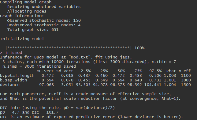
What inferences can we make from this output? The column named ‘muvect’ is similar to coefficient estimates in a basic linear model approach (the ‘lm()’ function in R). These are the means of each of the posterior distributions we estimated. 95% credible intervals for each parameter are displayed in the columns ‘2.5%’ and ‘97.5%’. Remember that these values represent a posterior distribution estimated from our 10,000 MCMC iterations. Usually, a parameter is considered “significant” if its 95% credible interval does not cross 0. You can see that both petal length and sepal width are “significantly” related to sepal length because their credible intervals do not cross 0. In other words, we are 95% confident that the mean parameter estimates for our variables fall within the 95% credible intervals displayed here. We had pretty good model convergence because all of our parameters have Rhat values very close to 1.
Okay, let’s see how our posterior means compare to a simple linear model with the same formula:
lmmod <- lm(Sepal.Length ~ Sepal.Width + Petal.Length, data=iris)
summary(lmmod)
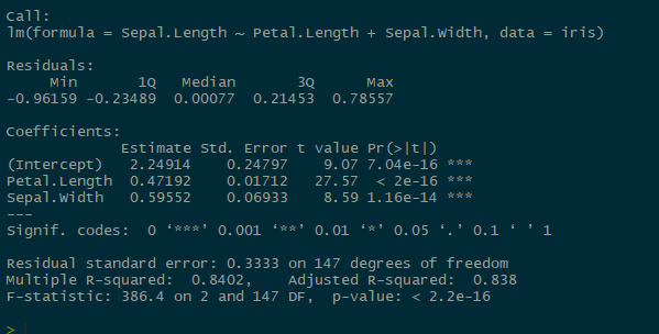
Our coefficient estimates almost match up exactly with our mean posteriors (mu.vect values) in the JAGS model! Not so difficult to interpret after all!
Hopefully you can use this mini-example as a starting-off point to write your own models in JAGS. Experiment with interaction terms, random effects, or non-linear functions if you like. Here are some individuals with good JAGS/BUGS tutorials that I pulled from for this blog: